How to Use the Spectral Analysis Tool in Sound Forge Pro
The Spectral Analysis tool in Sound Forge Pro is under View → Spectrum Analysis. It opens a frequency-domain view of whatever audio you have selected — amplitude on the vertical axis, frequency on the horizontal. FFT size, display mode, real-time monitoring, snapshot storage — all of it lives in that window. It's not a spectral editor; it doesn't let you paint out frequencies. It's a measurement and diagnostic tool, and knowing how to read it changes how you use EQ.
Quick answer: View → Spectrum Analysis → select audio → click Refresh (or enable Auto Refresh). For real-time monitoring during playback, click the Real-Time Monitoring button. The rest explains what the settings actually do and when each display mode is useful.
Spectrum Analysis, Spectroscope, WaveColor — Which Does What
Sound Forge Pro has three frequency visualization tools and people routinely mix them up.
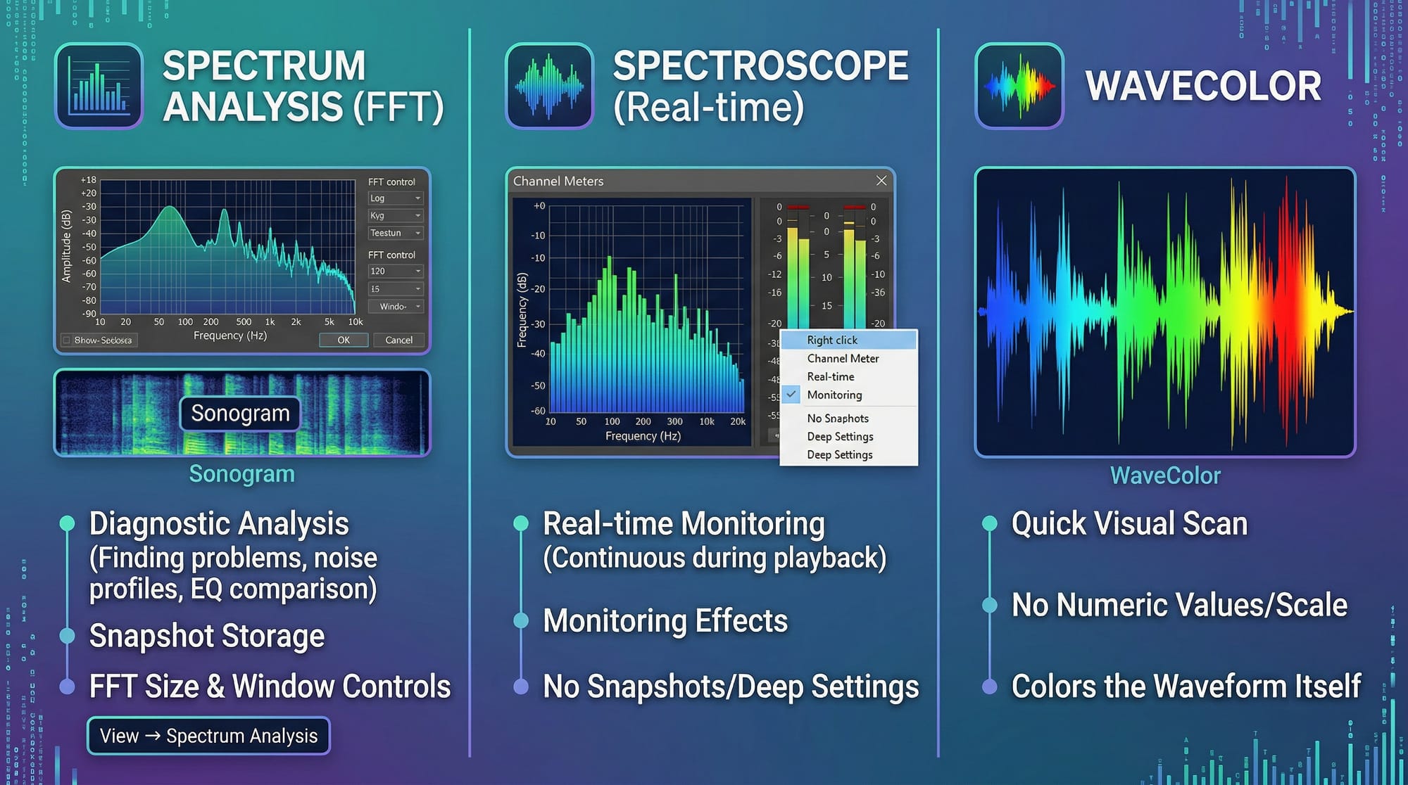
Spectrum Analysis (View → Spectrum Analysis) — the full FFT analysis window. Shows frequency content of a selection as a static or refreshed graph. Has FFT size controls, sonogram mode, snapshot storage. Primarily for diagnostic analysis: finding problem frequencies, comparing before/after EQ, identifying noise profiles.
Spectroscope — the real-time frequency meter, accessible via the Channel Meters panel (View → Channel Meters, then right-click the meters area). Shows frequency content continuously during playback. No snapshot, no settings depth. Useful for monitoring while applying effects and hearing what changes in real time.
WaveColor — not a separate window. It colors the waveform display itself: low frequencies show as one color, mids another, highs another. A quick visual scan before you open any analysis tool. No numeric values, no scale.
The article covers Spectrum Analysis specifically — the one with FFT controls and sonogram mode. On a vinyl restoration session last autumn I had all three open at once: WaveColor to spot where the crackle events were dense, Spectroscope to watch the noise floor in real time while NR was running, and Spectrum Analysis to compare snapshots before and after each pass. Each tool gave me something the other two didn't.
Opening Spectrum Analysis and Basic Navigation
Go to View → Spectrum Analysis. The window docks into the Sound Forge interface or floats — drag the title bar to position it. It doesn't update automatically until you tell it to.
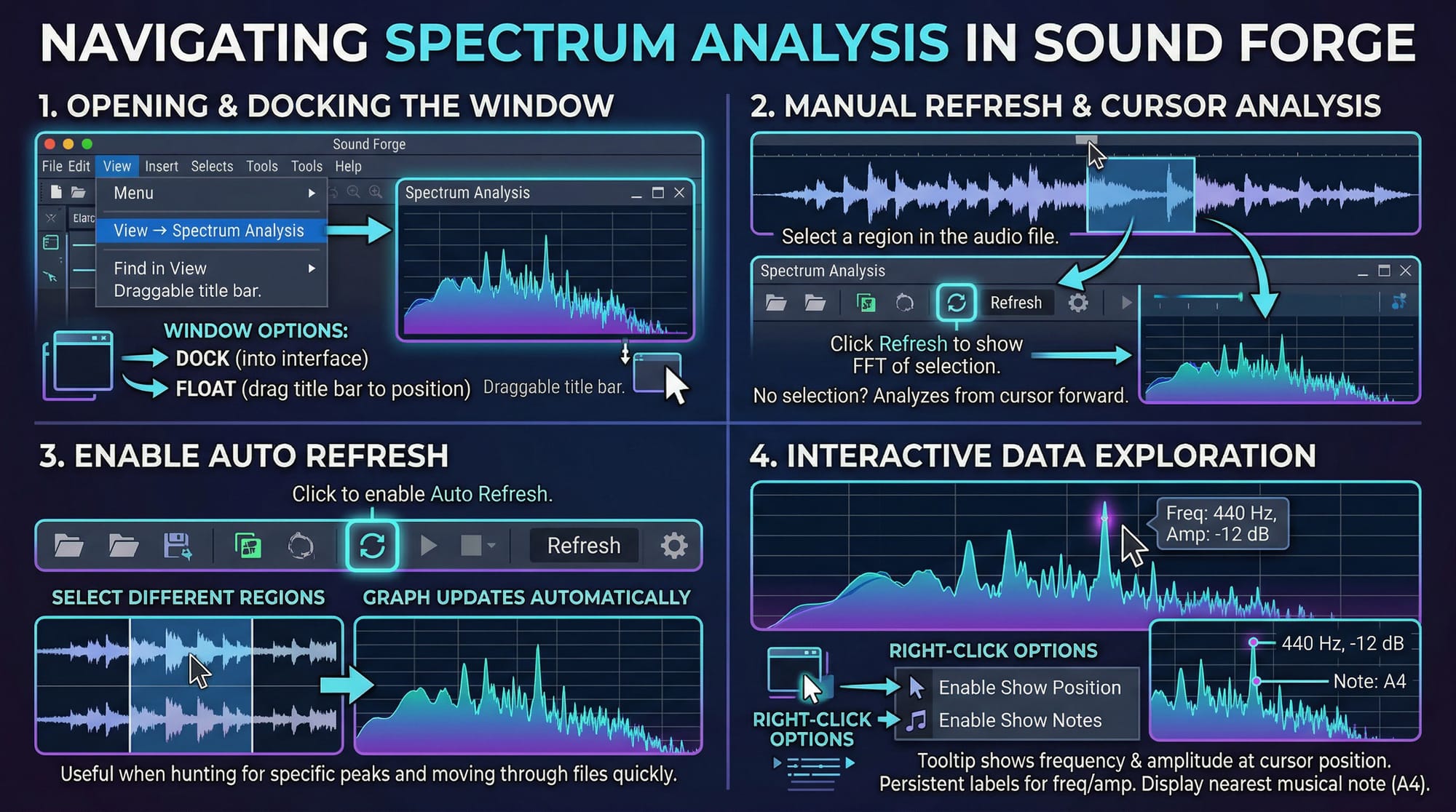
Select a region in your audio file, then click Refresh in the Spectrum Analysis toolbar. The graph updates to show the FFT of your selection. If no selection exists, it analyzes from the cursor position forward. Enable Auto Refresh (the button with the circular arrow) and the display updates every time you change your selection — useful when you're hunting for something specific and moving through the file quickly.
Hover the cursor over any point in the spectrum graph. A tooltip shows the exact frequency and amplitude at that position. Right-click and enable Show Position to keep it visible. Right-click and enable Show Notes to display the nearest musical note — useful when you're analyzing a recording and need to identify a resonant peak in terms of pitch rather than Hz.
FFT Size: The Setting That Determines What You Can See
Click the Settings button in the Spectrum Analysis window. FFT Size is the first control worth understanding — everything else in the dialog is secondary to it.
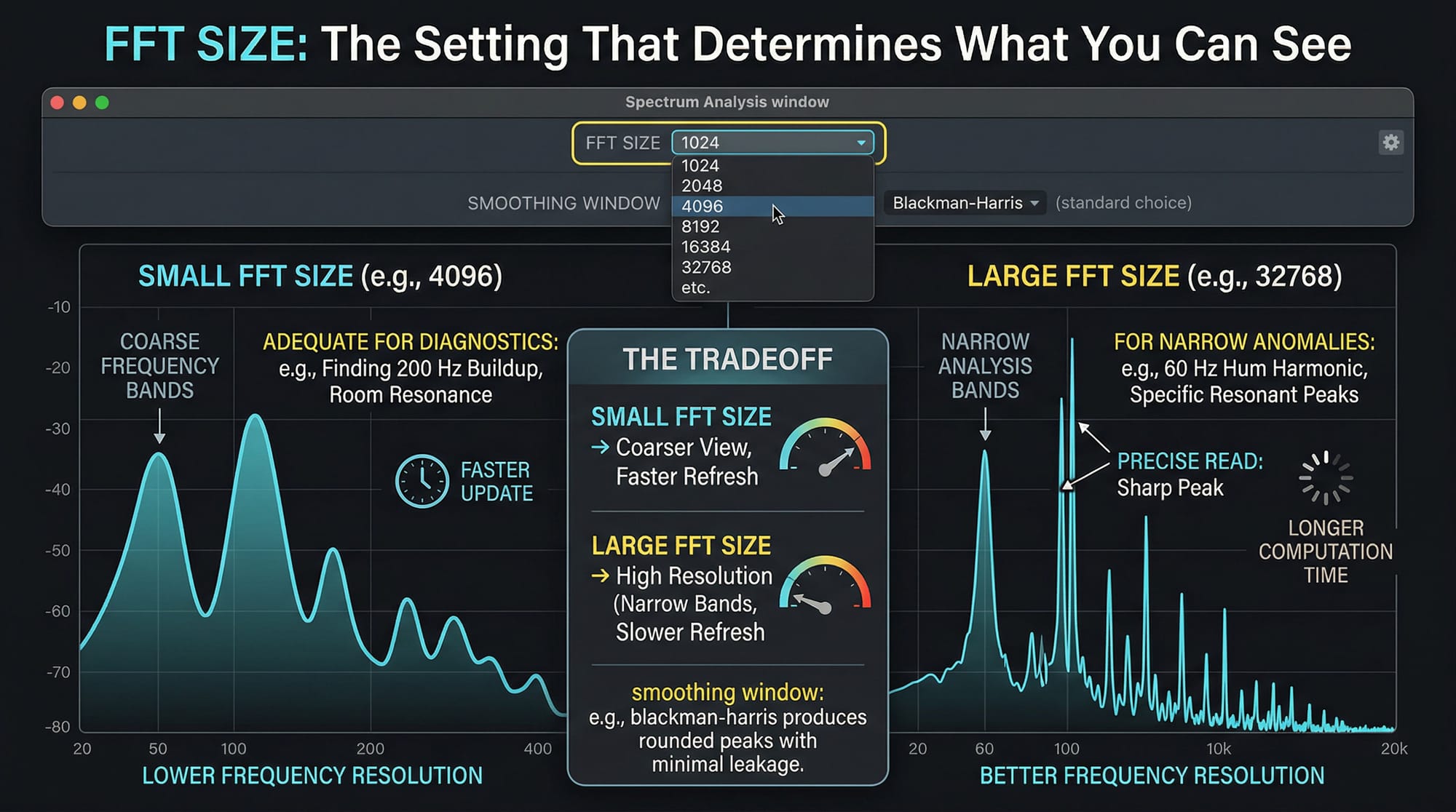
FFT size determines frequency resolution — how narrow the analysis bands are. Larger FFT size = better frequency resolution = longer computation time. Smaller = faster update, coarser frequency view.
For most diagnostic work — finding a buildup at 200 Hz, identifying a resonance in a room recording — FFT size 4096 or 8192 gives adequate resolution without sluggish display. For hunting narrow anomalies like a 60 Hz hum harmonic or a specific resonant peak in a mastered file, push it to 16384 or 32768. At those sizes the peaks become sharp enough to read precisely. The tradeoff is that the display takes longer to compute, so if you're refreshing frequently it gets slow. A practical breakdown of FFT size tradeoffs in audio work is in this Harmony Central guide on spectrum analysis.
The Smoothing Window setting affects how peaks are drawn. Blackman-Harris is the standard choice for audio — it produces rounded peaks with minimal leakage between adjacent frequency bands. Rectangular shows sharper peaks but with more inter-band leakage. Triangular sits between them. For most work, Blackman-Harris at 8192 is the starting point.
On a mastering session for a 9-track EP last year I ran Spectrum Analysis at FFT size 16384 on every file before touching EQ. Three of the nine had a sharp peak at 187 Hz that wasn't audible at normal listening levels but showed clearly in the graph. One notch filter per track, -2.5 dB each. They translated better on laptop speakers immediately.
Display Modes: Graph Types and Logarithmic Scale
Right-click the graph for display options.
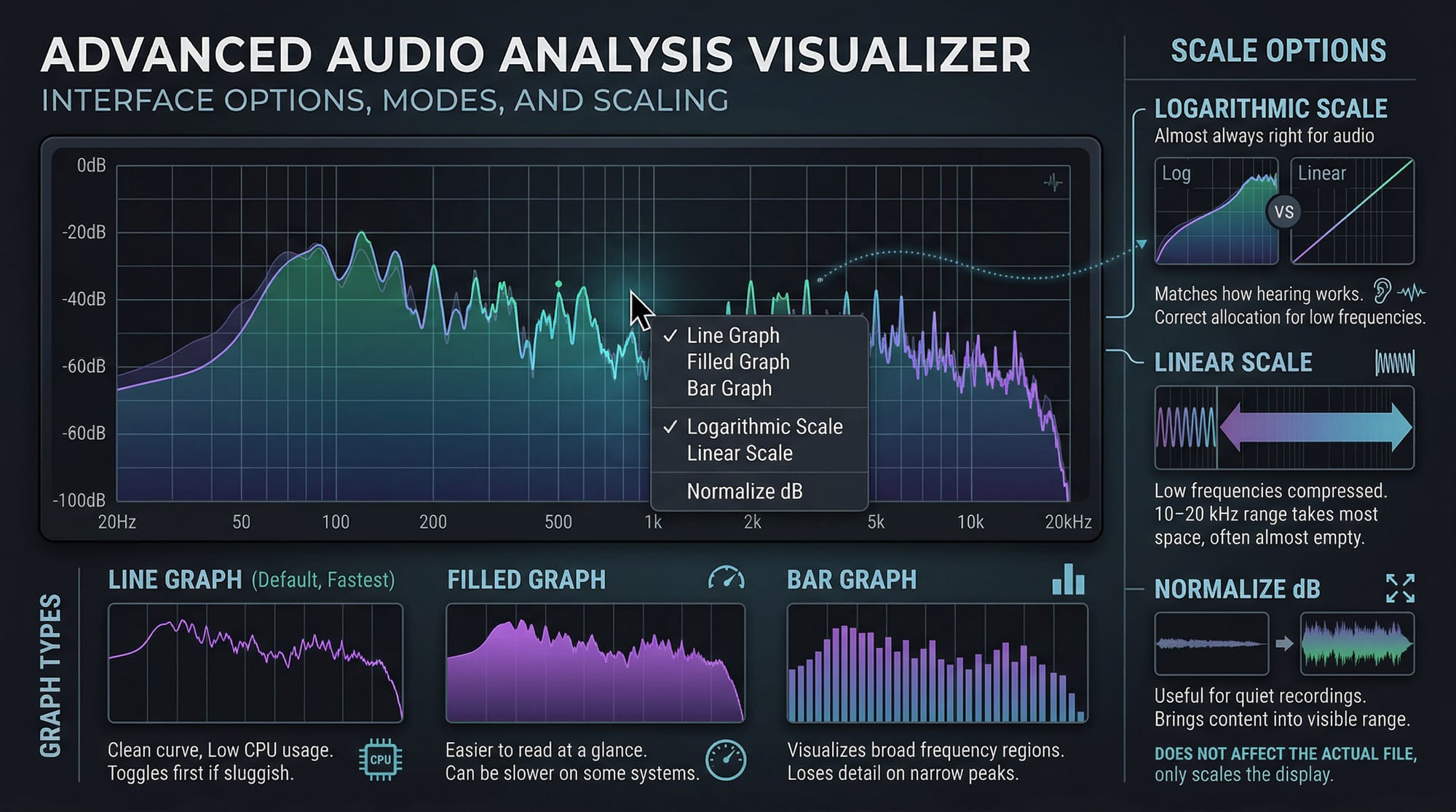
Line Graph is the default and fastest — clean frequency curve, low CPU. Filled Graph fills the area under the curve, easier to read at a glance but slower on some systems. Bar Graph shows frequency as discrete vertical bars — good for visualizing broad frequency regions but loses detail on narrow peaks. If the display feels sluggish, switch to Line Graph first.
Right-click and enable Logarithmic to toggle the X-axis between linear and log scale. Log mode is almost always the right choice for audio work — it allocates more space to lower frequencies, which matches how hearing actually works. Linear mode compresses the low-frequency region so severely that most of the graph is taken up by the 10–20 kHz range most recordings have almost nothing in.
Right-click and choose Normalize dB to scale the Y-axis to the actual range of your audio — useful when you're looking at a quiet recording and the peaks are buried in the bottom third of a -100 dB to 0 dB scale. Normalizing the display brings the content into the visible range without affecting the file.
Snapshots: The Feature Most People Skip
Sound Forge Pro's Spectrum Analysis stores up to four snapshots — frozen graphs you can overlay on the current analysis. Without this, you're relying on memory to compare what the frequency balance looked like before and after a processing step.
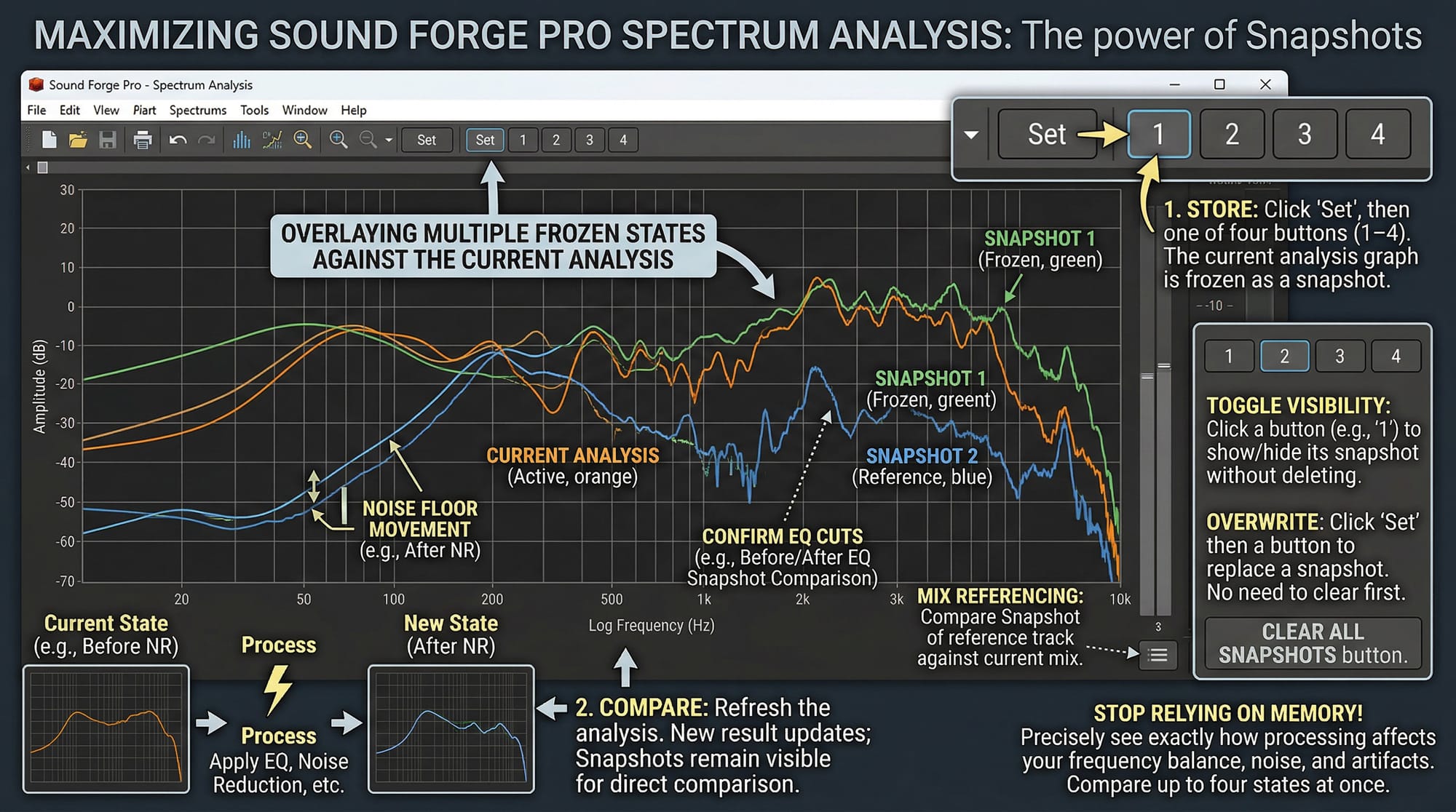
Click Set in the toolbar, then click one of the four snapshot buttons (labeled 1–4). The current graph is stored. Apply an EQ or other process, refresh the analysis, and the snapshot from before remains visible alongside the new result. You can compare four different states at once.
Snapshot before NR, run noise reduction, refresh and compare — see exactly how much the noise floor moved and whether you introduced any spectral artifacts. Snapshot before EQ, apply a cut, compare. Snapshot a reference track, then analyze your own mix in the same window — see where they diverge.
To hide individual snapshots without deleting them, click the snapshot button again to toggle it off. Click Clear All Snapshots to wipe them. You don't need to erase to overwrite — just click Set and then the snapshot button to replace it.
The Sonogram: Time and Frequency Together
Click the Sonogram button in the Spectrum Analysis window to switch from the standard spectrum graph to sonogram view. The axes change: time runs left to right on the X-axis, frequency runs bottom to top on the Y-axis, and amplitude is shown as color intensity. Brighter or more saturated = louder at that frequency at that moment in time.
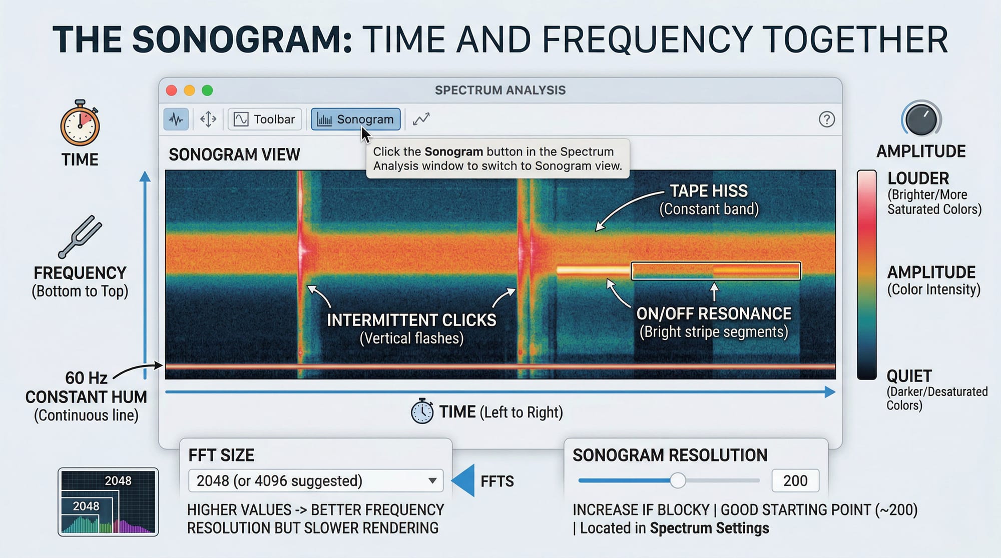
The sonogram makes time-varying frequency content visible in a way the standard spectrum graph can't. A 60 Hz hum that's constant shows as a continuous horizontal line at the bottom. An intermittent click appears as a vertical flash across all frequencies. Tape hiss appears as a constant mid-to-high frequency band. A resonance that only appears during certain passages shows as a bright horizontal stripe that turns on and off.
FFT size still applies in sonogram mode — higher values give better frequency resolution but slower rendering. For sonogram work, FFT size 2048 or 4096 is usually enough unless you need to distinguish very close frequencies. Increase the Sonogram Resolution setting in Spectrum Settings if the display looks blocky — around 200 is a good starting point, per the official docs.
Color or black-and-white: both available via right-click on the sonogram. Color mode makes amplitude differences more visible at a glance; B&W works better for printing or when you're screenshotting for documentation.
Real-Time Monitoring
Click the Real-Time Monitoring button and Sound Forge continuously updates the Spectrum Analysis display during playback. The dropdown under that button lets you choose between monitoring the input signal (useful when recording) or the output signal (useful when monitoring effects during playback through the Plug-In Chainer).
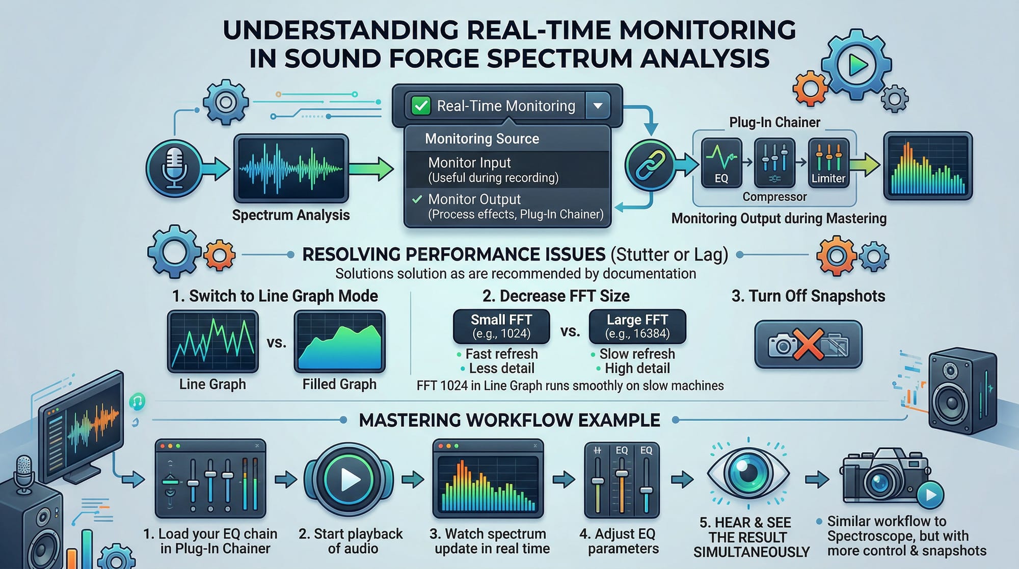
Real-time monitoring requires processing power. If playback stutters or the spectrum display lags badly, the helpmax documentation suggests three fixes: switch to Line Graph display mode, decrease the FFT size, or turn off snapshots. All three reduce the computational load on the display refresh. On a slower machine, FFT size 1024 in Line Graph mode with no snapshots will run smoothly where 16384 in Filled Graph mode won't.
Monitoring output through the Plug-In Chainer is useful during mastering: load your EQ chain, start playback, watch the spectrum update in real time, adjust the EQ while hearing and seeing the result simultaneously. This is the workflow the Spectroscope handles too, but Spectrum Analysis gives you more control over the display and the ability to snapshot a state for comparison.
What Spectrum Analysis Won't Do
It's a viewer, not an editor. You can identify that there's a peak at 340 Hz in a recording, but you can't select it and remove it from within Spectrum Analysis. You take that information to your EQ and make the cut there. For actual spectral editing — selecting and painting out specific frequencies while preserving others — you need SpectraLayers Pro (included in the Sound Forge Pro Suite) or iZotope RX Advanced. The noise reduction guide covers what the bundled NR tools can handle and where their limits are.
For a full view of how Spectrum Analysis fits into a mastering chain alongside Wave Hammer, EQ, and Statistics, the mastering guide covers the sequence. Spectrum Analysis belongs at the start — before any processing, to understand what you're working with. Then again after each processing step to confirm what changed.
Frequently Asked Questions
Where is the Spectral Analysis tool in Sound Forge Pro?
View → Spectrum Analysis. It opens a dockable or floating window. The Spectroscope (real-time frequency meter) is in the Channel Meters panel — View → Channel Meters, then right-click the meters area to add it. Separate tool, different purpose: Spectrum Analysis is for detailed FFT analysis with snapshot storage and sonogram mode; Spectroscope is for continuous real-time monitoring during playback.
What FFT size should I use in Sound Forge Pro Spectrum Analysis?
For general EQ analysis: 4096 or 8192. For hunting narrow anomalies like specific resonances or hum harmonics: 16384 or 32768. For real-time monitoring where CPU is limited: 1024 or 2048. Higher FFT size = better frequency resolution but slower display refresh. Blackman-Harris smoothing window is the standard starting point for most audio work.
What is the difference between the spectrum graph and the sonogram in Sound Forge Pro?
The spectrum graph shows amplitude vs. frequency at a single moment (or averaged over a selection) — a snapshot of frequency content. The sonogram shows amplitude vs. frequency vs. time — frequency on the Y-axis, time on the X-axis, amplitude as color intensity. The sonogram reveals how frequency content changes over time; the spectrum graph gives a cleaner, more precise view of the frequency distribution at a specific moment.
How do I compare before and after EQ in Sound Forge Pro Spectrum Analysis?
Take a snapshot before applying EQ: select your audio, open Spectrum Analysis, click Set, then click snapshot button 1. Apply the EQ. Select the same audio region again, click Refresh. The original snapshot remains visible in the graph alongside the new analysis. Up to four snapshots can be stored simultaneously for multi-stage comparison.
Does Sound Forge Audio Studio have a Spectrum Analysis tool?
No — Spectrum Analysis is a Sound Forge Pro feature. Audio Studio has basic audio restoration tools but not the full FFT analysis window. If you're on Audio Studio and need spectrum analysis, Voxengo SPAN is a free VST that provides real-time frequency analysis and loads through the Effects chain. For anything beyond basic analysis, the Sound Forge Pro review covers what Pro adds over Audio Studio.
How do I use Spectrum Analysis for mastering in Sound Forge Pro?
Run Spectrum Analysis at FFT size 8192–16384 on the full file before any processing. Look for: low-frequency buildups below 100 Hz, peaks in the 200–400 Hz range that cause muddiness, harshness between 2–5 kHz. Take a snapshot. Apply EQ corrections. Refresh and compare with the snapshot. Repeat after each processing step. The official Spectrum Analysis documentation covers every display option in detail.
Why is the Spectrum Analysis display sluggish or slow in Sound Forge Pro?
Real-time spectrum analysis is CPU-intensive. Three things that help: switch from Filled Graph to Line Graph display mode, decrease FFT size to 2048 or 1024, and turn off stored snapshots. If you're using real-time monitoring during playback, these three changes together usually resolve the lag. On older hardware, running Spectrum Analysis as a static refresh (no real-time monitoring) avoids the issue entirely.